Computer Modelling and Simulation Fundamentals

28th Jan 2025
15 min read
Tags:
simulation,
Review

Updated on 29th Jan 2025
See changes

Overview

Introduction to Simulation

Definition: Simulation is the process of creating a model of a real-world system and conducting experiments to understand and predict its behavior.
Types of Simulation:
- Static Simulation: Models do not change over time (e.g., Monte Carlo methods).
- Dynamic Simulation: Models evolve over time based on system rules.
- Deterministic Simulation: No randomness, same inputs lead to the same outputs.
- Stochastic Simulation: Includes randomness, outputs vary.
- Continuous Simulation: System state changes continuously over time.
- Discrete Simulation: State changes at distinct points in time.
Static Simulation Examples: Basic probability calculations, risk analysis.

Simulation Advantages, Disadvantages, and Steps

Advantages:
- Allows experimentation without physical implementation.
- Identifies potential system improvements.
- Can analyze scenarios that are dangerous or impractical to test in real life.
Disadvantages:
- Requires extensive data collection and validation.
- Can be time-consuming and computationally expensive.
- Results are model-dependent and may not perfectly reflect reality.
Steps in Simulation:
1. Define the problem and objectives.
2. Develop a conceptual model.
3. Collect data and identify probability distributions.
4. Implement the model in simulation software.
5. Conduct simulation experiments and collect results.
6. Analyze the results and refine the model.
7. Validate and verify the model.
Dynamic Simulation Examples: Inventory control, climate modeling, traffic systems.

Discrete Event Simulation (DES)

Key Components:
- Entities: Objects that flow through the system (e.g., customers, machines).
- Attributes: Characteristics of entities (e.g., service time, arrival rate).
- Events: Occurrences that change the system state (e.g., arrival, departure).
- System State: Set of variables that define the system at a given time.
- Statistical Collectors: Tools to measure and analyze performance (e.g., waiting times, throughput).
Collection of Statistics: Helps in evaluating the efficiency of different configurations.
Hand Simulation: Step-by-step manual simulation to verify model logic before software implementation.

Model Verification and Validation

Verification: Ensuring the simulation model is correctly implemented.
Validation: Ensuring the model accurately represents the real system.
Techniques for Validation:
- Face validation (expert review)
- Historical data comparison
- Sensitivity analysis
Example: Simulating a Single-Server Queueing System:
- Customers arrive at a service desk based on an interarrival distribution.
- The server processes customers according to a service time distribution.
- Performance metrics: Average queue length, server utilization, customer waiting time.

Input Distribution Fitting

Why it Matters: Real-world processes have inherent variability, requiring statistical distribution modeling.
Common Probability Distributions:
- Exponential: Common for interarrival times.
- Normal: Used for processes following a bell-curve pattern.
- Uniform: Used for evenly distributed random variables.
- Poisson: Used for modeling event occurrence rates.
Techniques for Distribution Fitting:
- Histogram fitting
- Goodness-of-fit tests (Chi-Square, Kolmogorov-Smirnov test)
- Maximum likelihood estimation

Random Number Generators (RNG)

Purpose: Generates sequences of pseudo-random numbers for simulation experiments.
Common Methods:
- Linear Congruential Generator (LCG): Uses modular arithmetic.
- Mersenne Twister: High-quality random number generator used in modern simulations.
- Inverse Transform Sampling: Converts uniform random numbers to desired distributions.
Random Number Generators in Simulation Software: Built-in functions in AnyLogic, SimPy, Arena, etc.

Output Analysis - Terminating Simulations

Terminating Simulations:
- Have a natural stopping point (e.g., store closing, project duration).
- Require replication to obtain reliable statistical measures.
Performance Measures: Mean, variance, confidence intervals.
Techniques for Output Analysis:
- Replicated runs with different seeds.
- Confidence interval estimation.
- Analyzing run variability.

Output Analysis - Steady-State Simulations

Definition: Simulations that run indefinitely or until statistical stability is reached.
Key Metrics:
- System equilibrium state.
- Mean performance over time.
Techniques:
- Removing transient (warm-up) period.
- Using batch means method to estimate steady-state averages.
- Analyzing autocorrelation in simulation results.

Agent-Based Simulation (ABS)

Definition: Uses autonomous agents that interact with each other and their environment.
Applications:
- Social behavior modeling
- Traffic congestion analysis
- Market simulation
- Epidemic spread analysis
Components:
- Agents: Independent decision-making entities.
- Environment: Space where agents interact.
- Rules & Behaviors: Governs agent actions.

Using Agents for Complex Systems Evaluation

Why Use ABS?
- Captures emergent behaviors.
- Models decentralized decision-making.
- Incorporates adaptive learning mechanisms.
Application Areas:
- Smart city planning.
- Ecological system analysis.
- Economic modeling.

Multi-Agent Systems and Populations

Multi-Agent Systems (MAS): Simulations where multiple agents influence each other.
Key Principles:
- Autonomy: Agents operate independently.
- Communication: Agents share information.
- Adaptation: Agents learn and evolve.
Examples:
- Swarm intelligence (e.g., flocking birds, ant colony optimization).
- Self-organizing traffic control.
- Stock market trading models.

Quiz

Question 0x01

In order to provide realistic output, scientific models _________.

Incorporate all known variables in the real world
Must be accurate physical representations of a system
Use equations to describe every process within a system
Simplify the real world where appropriate

Answer 0x01

Simplify the real world where appropriate.

Question 0x02

Simulations in which one or more input variables are random are referred to as ______.

Stochastic simulation
Deterministic simulation
Discrete-event simulation
Dynamic simulation
Agent-based simulation

Answer 0x02

Stochastic simulation. In Deterministic, Variables are set and fixed. In Discrete-event, the simulation is based on discrete events (can be deterministic or stochastic). In Dynamic, the simulation is based on continuous time (can be deterministic or stochastic). In Agent-based, the simulation is based on the behavior of agents (can be deterministic or stochastic).

Question 0x03

The ______ distribution is the only continuous distribution that has the memoryless property. The ______. Distribution is the only discrete distribution that possesses the memoryless property.

Normal – Binomial
Exponential – Geometric
Poisson – Exponential
Geometric – Poisson

Answer 0x03

Exponential – Geometric. The memoryless property states that the probability of an event occurring in the next time period is independent of the time that has already elapsed. The Exponential and Geometric distributions are the only distributions that possess this property.

Question 0x04

A bank is an example of ____________ system, since __________________ variables e.g., the number of customers in the bank-change only when a customer arrives or finishes being served and departs.

continuous – flow
agent-based – state
discrete – flow
discrete – state

Answer 0x04

discrete – state. In a discrete-state system, the state of the system changes only at discrete points in time. In a discrete-flow system, the state of the system changes continuously over time.

Question 0x05

In the ______________________________ simulation model inputs to the simulation are known values, while in the _____________________________ simulation model, one or more random variables are used for input data.

Answer 0x05

deterministic stochastic

Question 0x06

The future-event list (FEL) is typically represented by a ______________________________, which can be efficiently implemented using a _______________________________.

Answer 0x06

priority queue heap

Question 0x07

The exponential distribution has the memoryless property, meaning that _________________________________________________________________________.

Answer 0x07

the probability of an event occurring in the next time period is independent of the time that has already elapsed.

Question 0x08

Monte Carlo simulations calculate _________________________ probability, which can be used as an approximation of __________________________ probability when the number of trials is high enough.

Answer 0x08

empirical theoretical

Question 0x09

The multiplicative congruential generator $X_{i+1} = (3X_i) \mod 2^{32}$ will have a period of $2^{32}$. (T/F)

Answer 0x09

False. The period of this generator is $2^{32-2}$.

Question 0x0A

Match the Questions

Building the right model
Building the model right
Time to reach initial transient
Iterative correction procedure of model building
Specification of probability distributions in model building
If the arrival rate is not affected by the number of customers being served and waiting, the model is called

With the following answers

Infinite population model, input modeling, verification, calibration, validation, warm-up period.

Answer 0x0A

Building the right model - input modeling
Building the model right - verification
Time to reach initial transient - warm-up period
Iterative correction procedure of model building - calibration
Specification of probability distributions in model building - input modeling
If the arrival rate is not affected by the number of customers being served and waiting, the model is called - infinite population model

Question 0x0B

Explain the differences between discrete-event, agent-based, and continuous simulation paradigms.

Answer 0x0B

Discrete-event simulation is based on discrete events, such as the arrival of a customer at a bank or the completion of a service. Agent-based simulation is based on the behavior of agents, such as people or animals. Continuous simulation is based on continuous time, such as the flow of water in a river.

Question 0x0C

What are the differences between traditional programming and agent-based modeling approach? Give an example.

Answer 0x0C

Traditional programming is based on algorithms, while agent-based modeling is based on the behavior of agents. For example, a traditional program might calculate the average number of customers in a bank, while an agent-based model might simulate the behavior of individual customers in the bank.

Question 0x0D

What are the main characteristics of Agent-Based Modeling? Explain and give an example.

Answer 0x0D

Agent-based modeling is based on the behavior of agents, such as people or animals. Agents can interact with each other and with their environment. For example, an agent-based model of a traffic system might simulate the behavior of individual cars on a road, including how they interact with each other and with traffic lights.

Question 0x0E

Explain the differences between:

Dynamic simulation and static (Monte Carlo) simulation,
Deterministic simulation and stochastic simulation,
Discrete simulation and continuous simulation.

Answer 0x0E

Dynamic simulation is based on continuous time, while static (Monte Carlo) simulation is based on discrete events. For example, a dynamic simulation might model the flow of water in a river, while a static simulation might model the arrival of customers at a bank.

Deterministic simulation uses fixed input values, while stochastic simulation uses random input values. For example, a deterministic simulation might model the behavior of a machine with fixed parameters, while a stochastic simulation might model the behavior of a machine with random parameters.

Discrete simulation is based on discrete events, such as the arrival of a customer at a bank, while continuous simulation is based on continuous time, such as the flow of water in a river.

Question 0x0F

Give brief answers to the following questions:

What is the difference between model verification and validation?
Discuss why validating a model of a computer system might be easier than validating a military combat model. Assume that the computer system of interest is similar to an existing one.

Answer 0x0F

Model verification is the process of ensuring that a model is correctly implemented, while model validation is the process of ensuring that a model is an accurate representation of the real system.

Validating a model of a computer system might be easier than validating a military combat model because the computer system of interest is similar to an existing one. This means that the model can be compared to the existing system to ensure that it is accurate. In contrast, a military combat model might be more difficult to validate because it is based on hypothetical scenarios that have not yet occurred.

Question 0x10

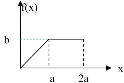
In a given probability density function “a” is a constant.

diagram

Find b in terms of a.
Find cdf of the variable X.
Find the expected value of the variable X.

Answer 0x10

Find b in terms of a. $$ \textrm{Total Area} = \frac{1}{2} a \cdot b + a \cdot b = \frac{3}{2} a \cdot b \newline \textrm{Since } f(x) \textrm{ is a probability distribution function, } \int_{-\infty}^{\infty} f(x) dx \textrm{ must be 1. So; } \newline \int_{-\infty}^{\infty} f(x) dx = \frac{3}{2} a \cdot b = 1 \rightarrow b = \frac{2}{3a} $$

Find cdf of the variable X. $$ f(x) = \begin{cases} \frac{b}{a}x, & \text{if } 0 \leq x \leq a \newline b, & \text{if } a \leq x \leq 2a \newline 0, & \text{o/w} \end{cases} $$

$$ F(x) = \int_0^x \frac{b}{a} x ,dx = \frac{b}{2a} x^2 \Big|_0^x = \frac{b}{2a} x^2, \quad \text{if } 0 \leq x \leq a $$

$$ F(a) = \frac{ab}{2} $$

$$ F(x) = F(a) + \int_a^x b ,dx = \frac{ab}{2} + bx \Big|_a^x = \frac{ab}{2} + bx - ab = bx - \frac{ab}{2}, \quad \text{if } a < x \leq 2a $$

$$ F(x) = \begin{cases} \frac{b}{2a} x^2, & 0 \leq x \leq a \newline bx - \frac{ab}{2}, & a < x \leq 2a \newline 1, & x > 2a \end{cases} $$

Find the expected value of the variable X. $$ E(x) = \int_{-\infty}^{\infty} x f(x) ,dx = \int_0^a x \frac{b}{a} x ,dx + \int_a^{2a} x b ,dx $$

$$ = \frac{b}{3a} x^3 \Big|_0^a + \frac{b}{2} x^2 \Big|_a^{2a} $$

$$ = \frac{ba^2}{3} + 2ba^2 - \frac{ba^2}{2} = \frac{11ba^2}{6} $$

Question 0x11

For each of the systems listed, sketch the logic of an event-oriented model. Develop the model in any language (or pseudocode):

A central-server queuing model: when a job leaves the CPU queue, it joins the I/O queue with shortest length.
A queuing model of database system that implements fork join: a job receives service in two parts. When it first enters the server it spends a small amount of simulation time generating a random number of requests to disks. It then suspends (freeing the server) until such time as all the requests it made have finished, and then enqueues for its second phase of service, where it spends a larger amount of simulation time, before finally exiting. Disks may serve requests from various jobs concurrently, but serve them using FCFS ordering. Your model should report on the statistics of a job in service – how long (on average) it waited for phase 1, how long it waits on average for its I/O requests to complete, and how long it waits on average for service after its I/O requests complete.

Answer 0x11

A central-server queuing model: when a job leaves the CPU queue, it joins the I/O queue with the shortest length.

from queue import PriorityQueue

class Job:
    def __init__(self, arrival_time, service_time):
        self.arrival_time = arrival_time
        self.service_time = service_time

    def __lt__(self, other):
        return self.service_time < other.service_time

class CentralServer:
    def __init__(self):
        self.cpu_queue = PriorityQueue()
        self.io_queue = PriorityQueue()

    def add_job(self, job):
        self.cpu_queue.put(job)

    def process_jobs(self):
        while not self.cpu_queue.empty():
            job = self.cpu_queue.get()
            self.io_queue.put(job)

central_server = CentralServer()
job1 = Job(0, 5)
job2 = Job(1, 3)
job3 = Job(2, 4)
central_server.add_job(job1)
central_server.add_job(job2)
central_server.add_job(job3)
central_server.process_jobs()

A queuing model of a database system that implements fork join.

from queue import PriorityQueue

class Job:
    def __init__(self, arrival_time, service_time):
        self.arrival_time = arrival_time
        self.service_time = service_time

    def __lt__(self, other):
        return self.service_time < other.service_time

class DatabaseSystem:
    def __init__(self):
        self.server_queue = PriorityQueue()
        self.disk_queue = PriorityQueue()

    def add_job(self, job):
        self.server_queue.put(job)

    def process_jobs(self):
        while not self.server_queue.empty():
            job = self.server_queue.get()
            self.disk_queue.put(job)

database_system = DatabaseSystem()
job1 = Job(0, 5)
job2 = Job(1, 3)
job3 = Job(2, 4)
database_system.add_job(job1)
database_system.add_job(job2)
database_system.add_job(job3)
database_system.process_jobs()

Question 0x12 to Question 0x14

MISSING

Question 0x15

Discuss why validating a model of a computer system might be easier than validating a military combat model. Assume that the computer system of interest is similar to an existing one.

Answer 0x15

A computer system simulation model is discrete, stochastic, dynamic, whereas a military combat model is continuous, stochastic and dynamic. So, validating a large scale military combat simulation model needs a finer (more detailed) but small scale simulation model.

Question 0x16

What are the differences between traditional programming and agent based modeling approach. Give an example.

Answer 0x16

ABM	Traditional Programming
Linear	Positive feedback is difficult to deal with
Correlation	Real mechanisms are not represented
Often static	Dynamics are not modeled
Emergence	Lower rules form patterns on higher levels
Self-organization	Program finds best pattern
Learning	Feedback is used to change behavior

Application Example: Market

ABM	Traditional Programming
Agents are located on a square grid	Agents are located on a square grid
They trade with their neighbours	They trade with their neighbours
There are two commodities: sugar and spice	There are two commodities: sugar and spice
All agents consume both these, but at different rates	All agents consume both these, but at different rates
Each agent has its own welfare function	Each agent has its own welfare function
Relating its relative preference for sugar or spice to the	Relating its relative preference for sugar or spice to the
amount it has ‘in stock’ and the amount it needs	amount it has ‘in stock’ and the amount it needs

Question 0x17

What are the main characteristics of Agent Based Modeling? Explain and give an example.

Answer 0x17

ABN is Decentralized.

There is no single place where the system's behavior is specified.
System’s behavior emerges from individual behavior of individual agents.

Example: Strop-and-go in front of a traffic light by individual cars results in wave characteristics of the traffic flow.

Global consequences of individual behavior in a given space.

ABM supports modeling of complexity.

If the interactions between parts are nonlinear, than the system cannot be simply described by the sum of its parts.

Application Example: Hampton Roads Traffic

Agent-based Modeling
- Individual behavior of drivers
  - Conservative drivers stay on their old route
  - Degree of driving education influences the through-put
- Merging lanes in front of bridges
- Aggressive versus passive drivers
  - Alternative Use
- Bridges are Agents
  - How well does a bridge feel (based on increased through-put, lower costs, etc.)
  - The “Bridge Agent” finds the best place to be

Recourses

AnyLogic in Three Days: Modeling and Simulation Textbook